Policy Gradient Theorem
Lecture notes from some of my coursework on reinforcement learning. I also highly recommend [Russell, and Norvig, (2016), Sutton, (2018)].
Reinforcement learning algorithms can be classified into two categories. Ones that obtain policies by estimating the value function (value-based methods), and ones that obtain policies directly via environment interaction (policy search methods). The policy gradient theorem [Sutton, et al. (1999)] is a foundational result that relates the gradient of the agent’s performance (the maximisation objective) to the gradient of its current policy. This means that given a parametric policy, an optimisation problem can then be formulated to maximise the agent’s performance by changing the policy parameters. This result is the base of a large body of modern policy search algorithms (AC-methods, TRPO, PPO etc.).
Formally, the policy gradient theorem states that:
- Given a parametric policy \(\pi_{\theta}\) and some Markov Decision Process
- Assuming that all episodes start from a single start state \(s_0\) from which every action leads to a state sampled from a uniform distribution \(\rho(s_1)\)
- Defining the performance measure to be maximised \(J(\theta)\) as the value of this start state \(v_{\pi_{\theta}}(s_0)\)
- It can be shown that the gradient of the performance measure is proportional to the gradient of the policy
Where \(\mu\) is the occupancy measure given the policy and \(q_{\pi}\) is the action value function. Under this theorem, this gradient can now be defined in a form that is suitable for computation by experience (given an approximate action value \(q_{\pi}\)).
An Intuitive Proof
From [Sutton, (2018)] Ch. 13.
We start this proof by looking at the definition of the performance measure. As highlighted above, we assume that the MDP is episodic and all episodes start from a single start state \(s_0\). This is simply for mathematical convenience and any MDP can be modified to fit this condition. The “real” start states can just be thought to come out uniformly from \(s_0\). Given this, we define the performance measure as the state value of \(s_0\) under the parametric policy \(\pi_{\theta}\).
\[J(\theta) \doteq v_{\pi_{\theta}}(s_0)\]At the end of this proof we require an expression for \(\nabla_{\theta} J(\theta)\). Intuitively, it might appear that this gradient must involve the gradient of the value function and transition dynamics since the performance does depend on the action selection and the distribution of states that follow the selected action. However, the following result shows how the gradient of the performance measure only requires the gradient of the policy. Let us start by evaluating \(\nabla_{\theta} v_{\pi_{\theta}}(s)\) for any state \(s \in S\). From here on, we drop the subscript \(\theta\) and assume that the policy, value function, and all gradients are w.r.t \(\theta\). We also drop the discount factor \(\gamma\) throughout the proof.
The value function at a state is simply the expected value of the actions available from that state. Hence,
\[\nabla v_{\pi} (s) = \nabla [\sum_{a} \pi(a|s) q_{\pi}(s,a)]\]The gradient can be moved inside the summation and it can be split using the product rule,
\[= \sum_{a} [ \nabla \pi(a|s) q_{\pi}(s,a) + \pi(a|s) \nabla q_{\pi}(s,a)]\]The first inner term cannot be further expanded. The Bellman equation for the state value under a policy tells us that \(v_{\pi}(s) = \sum_{a} \pi(a \vert s) \sum_{s'} p(s' \vert s, a) (r + v_{\pi}(s'))\). This means that the action value function \(q_{\pi}(a \vert s) = \sum_{s'} p(s' \vert s, a) (r + v_{\pi}(s'))\). We plug this into the second inner term.
\[\begin{align} &= \sum_{a} [ \nabla \pi(a|s) q_{\pi}(s,a) + \pi(a|s) \nabla \sum_{s'} p(s' | s, a) (r + v_{\pi}(s'))] \\ &= \sum_{a} [ \nabla \pi(a|s) q_{\pi}(s,a) + \pi(a|s) \sum_{s'} p(s' | s, a) (r + \nabla v_{\pi}(s'))] \end{align}\]\(\nabla v_{\pi}(s')\) can be unrolled in the exact same way to contain \(\nabla v_{\pi}(s'')\). It turns out that the gradient of the action value is progressively related to the next state’s value, and the next-to-next states value and so on. Meaning that it depends on the probability of visiting the next state and the next-to-next state. This unrolled quantity can be reduced to a probability such that
\[\nabla v_{\pi} (s) = \sum_{x \in S} \sum_{k=0}^{\infty} Pr(s \to x, k, \pi) \sum_{a} \nabla \pi(a|s) q_{\pi}(s, a)\]Where \(Pr(s \to x, k, \pi)\) is the probability of transitioning from state \(s\) to state \(x\) in \(k\) steps under policy \(\pi\). Meaning that \(\sum_{k=0}^{\infty} Pr(s \to x, k, \pi)\) is the number of time steps that a policy visits a state \(s\) in one episode on average.
Having derived this sub-result, we come back to the gradient of the performance measure.
\[\begin{align} J(\theta) &\doteq v_{\pi_{\theta}}(s_0) \\ \nabla J(\theta) &= \nabla v_{\pi_{\theta}}(s_0) \end{align}\]Plugging in our previous sub-result and modifying the terms given that \(s_0\) is the initial state,
\[\nabla v_{\pi_{\theta}}(s_0) = \sum_{s} \sum_{k=0}^{\infty} Pr(s_0 \to s, k, \pi) \sum_{a} \nabla \pi(a|s) q_{\pi}(s, a)\]Here \(\sum_{k=0}^{\infty} Pr(s_0 \to s, k, \pi)\) is the same probability evaluated from state \(s_0\) (let’s call this \(\eta(s)\)). In episodic tasks the on-policy distribution \(\mu(s) = \frac{\eta(s)}{\sum_{s'}\eta(s')}\). Since \(\eta\) is not directly known, we convert the equality into a proportionality by arranging \(\eta(s)\) as \(\eta(s')\) and \(\mu(s)\).
\[\begin{align} &= \sum_{s'} \eta(s') \sum_{s} \frac{\eta(s)}{\sum_{s'}\eta(s')} \sum_{a} \nabla \pi(a|s) q_{\pi}(s, a) \\ &= \sum_{s'} \eta(s') \sum_{s} \mu(s) \sum_{a} \nabla \pi(a|s) q_{\pi}(s, a) \\ \nabla J(\theta) \: &\propto \: \sum_{s} \mu(s) \sum_{a} \nabla \pi(a|s) q_{\pi}(s, a) \end{align}\]Early Policy Search Algorithms (REINFORCE)
Having obtained the policy gradient theorem, how can we use this result to obtain a learning algorithm? Here we briefly look at REINFORCE [Williams, (1992)] as an exercise to understand how this result can be converted into an algorithm.
Notice that in the final result, we sum over all possible states in the MDP and then multiply the inner terms with the likelihood of those states \(\mu(s)\). This summation and multiplication is not done explicitly under \(\pi\). However, we can now change this summation and multiplication into an expectation by computing the expectation of the inner terms explicitly under \(\pi\). Meaning that \(\sum_{s} \mu(s)\) turns into \(\mathbb{E}_{\pi} [ ... ]\) where the states and actions in the expectation are obtained under the policy \(\pi\) (where previously only the value function was computed under \(\pi\)). Doing this naturally also turns the proportionality in the result to an equality. Hence an unconditioned the sum over the occupancy measure turns into an expectation over the states obtained by rolling out the policy. This is a minor nuance but I think it’s one that is often omitted. In the following lines, we replace \(s\) and \(a\) with \(S_t \sim \pi\) and \(A_t \sim \pi\).
\[\begin{align} \nabla J(\theta) \: &\propto \: \sum_{s} \mu(s) \sum_{a} \nabla \pi_{\theta}(s,a) q_{\pi_{\theta}}(s, a) \\ &= \mathbb{E}_{\pi_{\theta}} [ \sum_{a} \nabla \pi_{\theta}(a|S_t) q_{\pi_{\theta}}(a, S_t) ] \end{align}\]Similarly, the sum over actions can also be converted into an expectation over \(\pi\) by multiplying and dividing the terms by \(\pi_{\theta}(a \vert S_t)\)
\[= \mathbb{E}_{\pi_{\theta}} [ \sum_{a} \frac{\pi_{\theta}(a|S_t)}{\pi_{\theta}(a|S_t)} \nabla \pi_{\theta}(a|S_t) q_{\pi_{\theta}}(a, S_t) ]\]Rewriting the sum over actions as an expectation (and replacing \(a\) with \(A_t\) for the same reasons as above)
\[= \mathbb{E}_{\pi_{\theta}} [\frac{q_{\pi_{\theta}}(A_t, S_t)}{\pi_{\theta}(A_t|S_t)} \nabla \pi_{\theta}(A_t|S_t) ]\]The expectation over the return (\(G_t\)) from a state and action is just the action value by definition (\(\mathbb{E}_{\pi_{\theta}} [G_t \vert S_t, A_t]\)). Hence, we can also replace \(q_{\pi_{\theta}}(A_t, S_t)\) by \(G_t\).
\[= \mathbb{E}_{\pi_{\theta}} [\frac{G_t}{\pi_{\theta}(A_t|S_t)} \nabla \pi_{\theta}(A_t|S_t) ]\]Finally, \(\frac{\nabla \pi_{\theta}(A_t \vert S_t)}{\pi_{\theta}(A_t \vert S_t)}\) is just \(\nabla \ln \pi_{\theta}(A_t \vert S_t)\). This gives us the final expression
\[\nabla J(\theta) = \mathbb{E}_{\pi_{\theta}} [G_t \nabla \ln \pi_{\theta}(A_t|S_t)]\]Looking at the final result, we have now related the gradient of our performance measure to quantities that can solely be obtained from environment interactions. \(\mathbb{E}_{\pi_{\theta}} [G_t]\) can be approximated by a summation over a sufficient number of samples (\(\frac{1}{n} \sum_{i=1}^n R_t\)) which means
\[\nabla J(\theta) \approx \frac{1}{n} \sum_{i=1}^n (R_t \nabla \ln \pi_{\theta}(A_t|S_t))\]REINFORCE is a Monte-Carlo policy gradient algorithm, meaning that \(G_t\) is approximated by obtaining Monte-Carlo rollouts. Several other algorithms have been derived from this idea by changing the way in which the return is approximated. Other interesting algorithmic changes have been introduced by the addition of baselines, critics (value fn. baselines), trust regions etc. I end this post with the REINFORCE pseudocode.
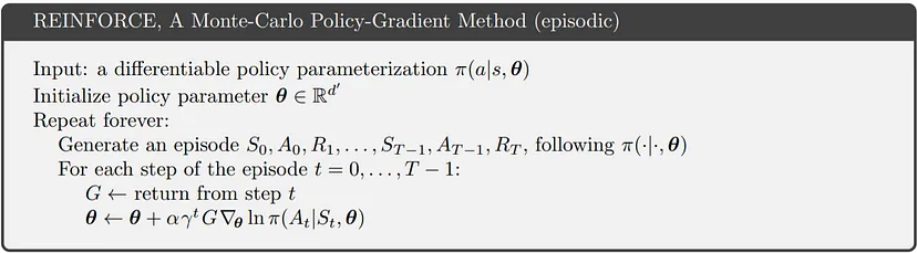
REINFORCE pseudocode.
References
Williams, Ronald J (1992). Simple statistical gradient-following algorithms for connectionist reinforcement learning. Machine learning
Sutton, Richard S and McAllester, David and Singh, Satinder and Mansour, Yishay (1999). Policy gradient methods for reinforcement learning with function approximation. Advances in neural information processing systems
Russell, Stuart J and Norvig, Peter (2016). Artificial intelligence: a modern approach.
Sutton, Richard S (2018). Reinforcement learning: An introduction. A Bradford Book