Monte Carlo Planning in Large Partially Observable MDPs
Decision-making (either human or artificial) typically involves taking actions given observations. For instance, (i) chess players make their move on observing the state of the board or (ii) driving agents take actions on observing the road and their surroundings. Naturally, the information encoded in these observations is pivotal to take the “right” actions. Partial observability is the situation when the agent’s observations do not completely represent all facets of information necessary to take actions. Looking back at our examples, (i) chess is a fully observable game since the agent observes all features necessary to take decisions whereas (a full observation is called the system’s state) (ii) driving could be thought of as a partially observable scenario since the agent might have visual blind spots 1. Partial observability is a feature of a dominant fraction of both real-world and conceptual decision-making problems — including problems such as autonomous driving, card games, robot navigation etc. — and leads to some very interesting challenges. In this post I will look at a planning framework in such a partially observable system.
Partially Observable MDPs
A Markov decision process [Sutton, (2018)] is a framework for modelling sequential decision making problems. It is founded on the Markov assumption that necessitates that state transitions are conditioned only on the current state and action and not on the history of actions. This implies that an agent is assumed to be perfectly capable of taking optimal actions only based on its knowledge of the current state (assuming that it has captured reward and transition dynamics via sufficient experience gathering).
The partially observable Markov decision process (POMDP) extends the standard MDP into the partially observable setting. A POMDP is defined as a 7-tuple \(\langle S , A , R , T , \Omega , O, \gamma \rangle\) where, as usual:
- \(S\) is a set of states, \(A\) is a set of actions, \(R(s, a)\) is the reward function, \(T(s, a, s') \triangleq P(s' \vert s, a)\) is the state transition function, and \(\gamma\) is the discount factor 2.
- Here the state \(s\) is not fully observable. Instead \(\Omega\) is a set of possible observations from which an observation \(o\) is sampled via some conditional observation probability \(O(o \vert s, a)\).
In a POMDP, we assume that the underlying system is still an MDP. However, the agent now does not have access to its true state \(s \in S\). It can only see the observation \(o \in O\). On taking an action \(a_t\) in true (but unknown) state \(s_t\), the agent transitions to the new state \(s_{t+1}\) with \(P(s_{t+1} \vert s_t, a_t)\) as usual. However, it does not directly see \(s_{t+1}\). Instead, the agent receives an observation \(o_{t+1} \in O\) which is conditioned on the new state and its previous action with \(P(o_{t+1} \vert s_{t+1}, a_t)\).
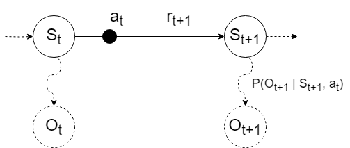
POMDP state transitions.
One strategy to deal with the uncertainty in the state is to keep track of a belief state, i.e, “which true states do I believe the system is in?”. Formally, the belief state is a distribution over the state space conditioned on the agent’s recent history of observations (other equivalent definitions of the belief state are conditioned over current belief and action-observation pair, however, this post uses the history definition). Belief state, \(B(h_t) \triangleq P(s_t \vert h_t)\) where \(h_t = [o_t, a_{t-1}, o_{t-1}, a_{t-2} ...]\). The other recursive definition of belief is \(b_t \triangleq P(s_t \vert a_t, o_t, b_{t-1})\). The belief state is integral to decision-making in POMDPs and can be considered almost a surrogate for the true state 3. The belief state can be calculated analytically (given the transition and observation models) through the application of the Bayes rule [Cassandra, et al. (1994)]. However, it can also be updated through data-driven approaches such as filtering (as will be seen in the next section on POMCP).
Partially Observable Monte-Carlo Planning (POMCP)
POMCP [Silver, and Veness, (2010)] is a heuristic search method for online planning in large POMDPs. It is a partial observability extension of one of the more popular model-based algorithms for solving large MDPs called UC-Trees [Kocsis, and Szepesv{'a}ri, (2006)] (which itself is an extension of Monte-Carlo Tree Search). POMCP combines Monte-Carlo belief state updates with a belief state version of UC-Trees to ensure tractability, even in large POMDPs. This section assumes a general understanding of MCTS.
Iterative planning algorithms that consider all states equally tend to perform quite poorly in large problems. The increased size of the state, action, or belief space leads to issues termed the curse of dimensionality and the curse of history. The former refers to the situation where the search space of the algorithm is simply too large for it to make any significant progress at estimating optimal solutions. The latter is a challenge specifically arising in belief-contingent problems where the number of possible action-observation histories grows exponentially with the horizon, leading to a very large possible solution search space. POMCP overcomes these challenges as it is a best-first method that rapidly focuses only on promising solution sub-spaces.
POMCP consists of two main subroutines. First, it uses partially observable UC-Trees (PO-UCT) to select actions at each time step in the real world. Second, it uses a particle filter and the simulated tree to update the agent’s belief state.
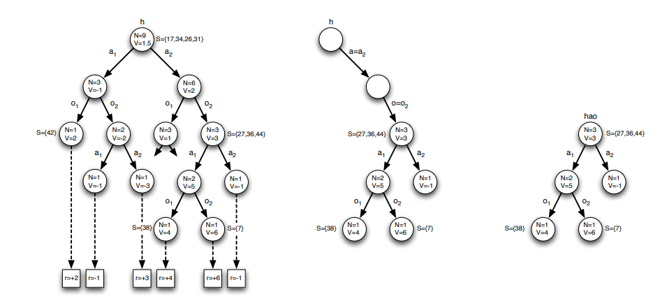
An illustration of POMCP in an environment with 2 actions, 2 observations, 50 states, and no intermediate rewards. The agent constructs a search tree from multiple simulations and evaluates each history by its mean return (left). The agent uses the search tree to select a real action and observes a real observation (middle). The agent then prunes the tree and begins a new search from the updated history (right) [Silver, and Veness, (2010)].
Unlike regular UCT, PO-UCT builds a search tree of histories instead of states. A history vector \(h_t\) is defined as \(ht = \{ a_1, o_1, ..., a_t, o_t \}\). The tree is rooted at the current history and contains a node \(T(h) = \langle N(h), V (h) \rangle\) for each represented history \(h\), where \(N(h)\) is the number of times each history \(h\) is visited and \(V(h)\) is its value (mean return from all simulation trajectories from \(h\)). Assuming that belief state \(B(s \vert h)\) is known exactly (this is later provided by the second subroutine), each simulation iteration starts from an initial state sampled from \(B(. \vert h)\) and performs tree traversal and rollouts just like standard UCT (with a UCB1 tree policy and then a history based rollout policy). After multiple iterations of the algorithm in simulation, the action that maximises value in the completed tree is selected as the real-world action.
The second subroutine of POMCP involves estimating the belief state through a particle filter. The belief state for history \(h_t\) is approximated by \(K\) particles, \(B_{i_t} \in S\) where \(1 \leq i \leq K\). Each particle is a belief and the belief state is the sum of all particles, \(B(s, h_t) = \frac{1}{K} \sum \delta_s B_{i_t}\). At the start of the algorithm, particles are sampled from the initial belief distribution. Particles are updated after the real-world action. During the simulation phase of the algorithm (first subroutine), a particle is added if the simulated observation in the iteration matches the last real-world observation. This is repeated until all \(K\) particles have been added and the belief state is complete. This is then repeated at every real-world step.
When search is complete, the agent selects the action at with the greatest value and receives a real observation \(o_{t+1}\) from the world. At this point, the node \(T(h_t, a_t, o_{t+1})\) becomes the root of the new search tree, and the belief state \(B(h_t, a_t, o_t)\) determines the agent’s new belief state. The remainder of the tree is then pruned as all past histories are now impossible.
References
Sutton, Richard S (2018). Reinforcement learning: An introduction. A Bradford Book
Cassandra, Anthony R and Kaelbling, Leslie Pack and Littman, Michael L (1994). Acting optimally in partially observable stochastic domains.
Silver, David and Veness, Joel (2010). Monte-Carlo planning in large POMDPs. Advances in neural information processing systems
Kocsis, Levente and Szepesvri, Csaba (2006). Bandit based monte-carlo planning.
-
The simplest way to deal with partial observability is to simply forget that it exists (often called the ostrich approach). You can always assume that the observations you get are the complete picture. In some cases like driving this is not a terrible assumption. In other cases like the game of poker, this is obviously incorrect. ↩
-
The discount factor is one of the defining features of the problem (not a feature of the decision making algorithm) because changing \(\gamma\) changes the optimal solution to the problem. ↩
-
A naive way to plan in POMDPs is to simply think of the POMDP as a new belief state MDP. ↩