Mirror Descent
Consider optimizing a differentiable, convex function $f: X \rightarrow \mathbb{R}$. Typical gradient descent (or projected subgradient descent) prescribes the update $x \gets x - \eta \nabla f(x)$. However, here, our assumption is that $X$ is a Euclidean space. In general, this geometric assumption that $\nabla f(x)$ is subtractable from $x$ is not true for different notions of distance. In the general setting, $\nabla f(x)$ maps points in $X$ to a dual space $X^\star$. Gradient descent’s $x - \eta \nabla f(x)$ update only works because $X^\star$ is isometric to $X$ in the Euclidean setting.
Mirror Descent (MD) is an optimization algorithm that adapts to potentially non-Euclidean geometrics, leveraging updates in the dual space, and often resulting in better results. This tutorial 1 walks through the MD optimization procedure in detail and shows an example of MD in the setting where $X$ is a simplex.
Introduction: Subgradient Descent
The MD optimization problem uses the first-order approximation 2 of a function with a promixity constraint. This construction is very similar to the simpler subgradient descent (MD mainly varies in the proximity term). Given an optimization iteration $t$, subgradient descent solves the optimization problem 3,
\[\begin{align*} x_{t+1} &= \underset{x \in X}{\arg \max} \quad \underbrace{f(x_t) + \langle g_t, (x-x_t) \rangle}_{\text{lin. approx.}} + \underbrace{\frac{1}{2 \eta} \left \lVert x - x_t \right \rVert_2^2}_{\text{prox.}} \\ &= \underset{x \in X}{\arg \max} \quad \eta \; \langle g_t, x \rangle + \frac{1}{2} \left \lVert x - x_t \right \rVert_2^2 \\ \\ &\text{where } g_t \in \partial f(x_t) \end{align*}\]The prox. term essentially ensures that our next iterate is not too far away from $x_t$, the point where our linear approximation is the least erroneous. The prox. term is defined based on the Euclidean norm in subgradient descent. Changing it allows us to work in spaces with different notions of distance. Typically, this change let’s us “rescale” space so that our updates are better aligned with the optimum.
Bregman Divergence: An alternate notion of distance
For a differentiable convex function $\varphi: \mathcal{D} \to \mathbb{R}$, the Bregman divergence is:
\[D_\varphi(x, y) = \underbrace{\varphi(x)}_{\text{value at x}} - \underbrace{\left[ \varphi(y) + \langle \nabla \varphi(y), x - y \rangle \right]}_{\text{lin. approx. of } \varphi \text{ at } y \text{ evaluated at } x}\]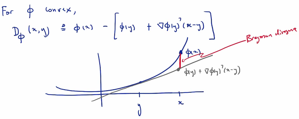
Illustration of the Bregman divergence (attribution: [Constantine Caramanis](https://youtu.be/UtoI5zsB3ZQ?si=6myuUVs9fla4iDBG))
Special Case: Bregman Divergence & KL Divergence
Take $\varphi$ to be the negative Shannon entropy on the probability simplex (componentwise on $x \in \Delta^n$):
\[\varphi(x) \;=\; \sum_{i=1}^n x_i \log x_i .\]Then \(\left(\nabla \varphi(y)\right)_i \;=\; 1 + \log y_i .\)
Plug into the Bregman formula:
\[D_\varphi(x,y) = \sum_i x_i \log x_i \;-\; \sum_i y_i \log y_i \;-\; \sum_i (1+\log y_i)\,(x_i-y_i).\]Expand the last term:
\[\sum_i (1+\log y_i)(x_i-y_i) = \sum_i (x_i-y_i) + \sum_i (x_i-y_i)\log y_i.\]If $x,y \in \Delta^n$, then $\sum_i x_i = \sum_i y_i = 1$, so $\sum_i (x_i-y_i)=0$. Hence
\[D_\varphi(x,y) = \sum_i x_i \log x_i \;-\; \sum_i y_i \log y_i \;-\; \sum_i (x_i-y_i)\log y_i = \sum_i x_i \log x_i \;-\; \sum_i x_i \log y_i.\]Therefore
\[D_\varphi(x,y) = \sum_{i=1}^n x_i \log\frac{x_i}{y_i} \;=\; \mathrm{KL}(x \,\|\, y).\]When optimizing over the simplex (probability vectors), choosing $\varphi(x)=\sum_i x_i\log x_i$ makes the “proximity term” in mirror descent be $\mathrm{KL}(x|y)$ rather than an $\ell_2$ distance. This matches the simplex’s geometry and yields iterates that stay in the simplex via exponentiated/multiplicative-style updates instead of Euclidean projection.
Mirror Descent (MD)
Special cases:
- $\varphi(x) = \frac{1}{2}|x|_2^2$ recovers projected gradient descent
- $\varphi(x) = \sum_i x_i \log x_i$ on simplex gives exponential/multiplicative weights
Requirements on $\varphi$:
- $\rho$-strongly convex w.r.t. some norm $|\cdot|$
- Differentiable on interior of domain $\mathcal{D}$
- $\nabla \varphi$ surjective
The choice of $\varphi$ determines the geometry of the algorithm, which norm appears in convergence guarantees, and the computational cost of updates. For a full convergence analysis refer here.
Primal-Dual Interpretation
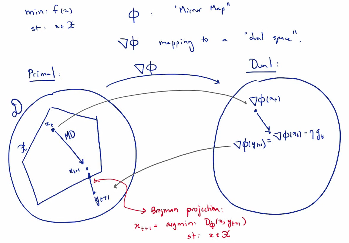
Illustration of the the primal-dual picture of MD (attribution: [Constantine Caramanis](https://youtu.be/UtoI5zsB3ZQ?si=6myuUVs9fla4iDBG))
Mirror descent can be viewed as alternating between primal and dual spaces.
Setup:
- Primal space: $X \subseteq \mathcal{D}$ (where $x_t$ lives)
- Dual space: $\nabla \varphi(\mathcal{D})$ (image of the gradient map)
- Mirror map: $\nabla \varphi: \mathcal{D} \to \nabla \varphi(\mathcal{D})$
Algorithm (unconstrained):
- Start in primal: $x_t$
- Map to dual: $\theta_t = \nabla \varphi(x_t)$
- Gradient step in dual: $\theta_{t+1} = \theta_t - \eta g_t$
- Map back to primal: $x_{t+1} = (\nabla \varphi)^{-1}(\theta_{t+1})$
With constraints: Step 4 becomes Bregman projection onto $X$.
Key insight: We never add gradients to primal points. The familiar update $x_t - \eta g_t$ only happens in dual space. This explains the “mirror” terminology — updates are reflected between spaces.
For negative entropy on simplex:
- Primal: $x \in \Delta_n$ (probabilities)
- Dual: $\theta_i = \log x_i + 1$ (log-probabilities)
- Dual update: $\theta_{t+1} = \theta_t - \eta g_t$ (linear in dual!)
- Back to primal: $x_{t+1,i} \propto e^{\theta_{t+1,i}}$ (exponential map)
Definitions & Analysis
-
$\ell_2$ is self-dual: $\lVert u \rVert_2 = \underset{\lVert v \rVert_2 \leq 1}{\max} \langle u, v \rangle$. The maximizer is $v = \frac{u}{\lVert u \rVert_2}$, giving $\lVert u \rVert _{\star} = \lVert u \rVert_2$.
-
$\ell_1$ and $\ell_\infty$ are dual:
-
$\ell_\infty$ is the dual of $\ell_1$: $\lVert u \rVert_\infty = \underset{\lVert v \rVert_1 \leq 1}{\max}\, \langle u, v \rangle$.
A maximizer is $v = \operatorname{sign}(u_{i^\star})\, e_{i^\star}$ where $i^\star \in \arg\max_i \left\lvert u_i \right\rvert$, giving $\langle u, v \rangle = \left\lvert u_{i^\star} \right\rvert = \lVert u \rVert_\infty$. -
$\ell_1$ is the dual of $\ell_\infty$: $\lVert u \rVert_1 = \underset{\lVert v \rVert_\infty \leq 1}{\max}\, \langle u, v \rangle$.
A maximizer is $v_i = \operatorname{sign}(u_i)$ for all $i$, giving $\langle u, v \rangle = \sum_i \left\lvert u_i \right\rvert = \lVert u \rVert_1$.
Key inequalities:
- Hölder’s inequality: $\left\lvert \langle u, v \rangle \right\rvert \leq \lVert u \rVert \cdot \lVert v \rVert_\star$ (equality when $v = \alpha \cdot \arg\max_{\lVert w \rVert \leq 1}\langle u, w \rangle$ for some $\alpha \ge 0$)
- Generalized Young’s inequality: $\langle u, v \rangle \leq \frac{1}{2\alpha}\lVert u \rVert^2 + \frac{\alpha}{2}\lVert v \rVert_\star^2$ for any $\alpha > 0$
Geometric interpretation: The gap between $\varphi(x)$ and its first-order Taylor approximation at $y$.
Properties:
- Non-negativity: $D_\varphi(x, y) \geq 0$ (by convexity)
- Not symmetric: Generally $D_\varphi(x, y) \neq D_\varphi(y, x)$
- Not a metric: Doesn’t satisfy triangle inequality
- Convex in first argument: $D_\varphi(\cdot, y)$ is convex
Examples:
-
Squared Euclidean distance: $\varphi(x) = \frac{1}{2}|x|_2^2$ \(D_\varphi(x, y) = \frac{1}{2}\|x\|_2^2 - \frac{1}{2}\|y\|_2^2 - \langle y, x-y \rangle = \frac{1}{2}\|x-y\|_2^2\)
-
KL divergence: $\varphi(x) = \sum_i x_i \log x_i$ on the simplex \(D_\varphi(x, y) = \sum_i x_i \log \frac{x_i}{y_i}\)
Useful identity: For any convex $\varphi$, \(\langle \nabla \varphi(x) - \nabla \varphi(y), x - z \rangle = D_\varphi(x, y) + D_\varphi(z, x) - D_\varphi(z, y)\)
Proof: Expand using the definition; all $\varphi$ terms cancel. $\square$
Equivalent characterizations:
- $\varphi(x) - \frac{\rho}{2}|x|^2$ is convex
- $D_\varphi(x, y) \geq \frac{\rho}{2}|x - y|^2$
Examples:
- $\varphi(x) = \frac{1}{2}|x|_2^2$ is 1-strongly convex w.r.t. $|\cdot|_2$
- Negative entropy $\sum_i x_i \log x_i$ is 1-strongly convex w.r.t. $|\cdot|_1$ on $\Delta_n$
Strong convexity ensures the Bregman divergence lower-bounds the squared distance.
If $f$ is convex, then for any $x,y$ we have the first-order condition of convexity
\[\begin{align*} f(y) &\;\geq\; f(x) + \langle \nabla f(x),\, y-x \rangle \\ f(x) - f(y) &\;\leq\; \langle \nabla f(x),\, x-y \rangle \\ \langle \nabla f(x),\, x-y \rangle &\;\leq\; \lVert \nabla f(x) \rVert_\star \,\lVert x-y \rVert \quad \text{ Holder ineq.} \\ \left\lvert f(x) - f(y) \right\rvert &\;\leq\; \lVert \nabla f(x) \rVert_\star \,\lVert x-y \rVert \\ \end{align*}\]Therefore, an equivalent way to state $L$-Lipschitzness w.r.t. $\lVert\cdot\rVert$ (for convex, differentiable $f$) is:
\[\lVert \nabla f(x) \rVert_\star \;\leq\; L \quad \text{for all } x.\](More generally, in the non-differentiable case: $\lVert g \rVert_\star \le L$ for all $g \in \partial f(x)$.)
Key consequence (quadratic upper bound / “fits a quadratic on top”):
\[f(y) \;\leq\; f(x) + \langle \nabla f(x),\, y-x \rangle + \frac{\beta}{2}\,\lVert y-x\rVert^2 \quad \text{for all } x,y.\]This is the non-Euclidean analogue of the usual smoothness inequality; only the norm changes, and the gradient side uses the dual.
Why this matters: smoothness quantifies how accurate the linear approximation is..
Applying MD to a Simplex
Consider minimizing $f$ over a simplex $\Delta_n = {x \geq 0: \sum_i x_i = 1}$ with $|\nabla f(x)|_\infty \leq 1$. This problem is very typical in reinforcement learning, where we wish to learn policies.
If we use $\varphi(x) = \sum_i x_i \log x_i$ (negative entropy on $\Delta_n$), we see the following:
Key properties:
- 1-strongly convex w.r.t. $|\cdot|_1$: Can be verified using the Hessian
- Gradient: $\nabla \varphi(x)_i = \log x_i + 1$
- Initial divergence: With $x_0 = (1/n, \ldots, 1/n)$, \(D_\varphi(x, x_0) = \sum_i x_i \log(nx_i) \leq \log n\)
Convergence: With $L = 1$ (in $\ell_\infty$, which is dual to $\ell_1$), $\rho = 1$, $R^2 = \log n$: \(f\left(\frac{1}{T}\sum_{t=1}^T x_t\right) - f(x^*) \leq \sqrt{\frac{2\log n}{T}}\)
Comparison:
| Method | Geometry | Convergence |
|---|---|---|
| Projected GD | Euclidean ($\ell_2$) | $O\left(\frac{\sqrt{n}}{\sqrt{T}}\right)$ |
| Mirror Descent | $\ell_1$ (negative entropy) | $O\left(\frac{\sqrt{\log n}}{\sqrt{T}}\right)$ |
The improvement from $\sqrt{n}$ to $\sqrt{\log n}$ is exponential in $n$.
The Exponential Weights Update
What does the mirror descent update look like on the simplex with negative entropy?
Starting from: \(x_{t+1} = \underset{x \in \Delta_n}{\arg\min} \left\{ \eta \langle g_t, x \rangle + D_\varphi(x, x_t) \right\}\)
First-order optimality: \(0 \in \eta g_t + \nabla \varphi(x_{t+1}) - \nabla \varphi(x_t) + N_{\Delta_n}(x_{t+1})\)
Unconstrained update: Define $y_{t+1}$ via: \(\nabla \varphi(y_{t+1}) = \nabla \varphi(x_t) - \eta g_t\)
For negative entropy, $\nabla \varphi(x)_i = \log x_i + 1$: \(\log y_{t+1,i} + 1 = \log x_{t,i} + 1 - \eta g_{t,i}\) \(y_{t+1,i} = x_{t,i} e^{-\eta g_{t,i}}\)
Normalization: Project back to simplex: \(x_{t+1} = \frac{y_{t+1}}{\|y_{t+1}\|_1} = \frac{(x_{t,1}e^{-\eta g_{t,1}}, \ldots, x_{t,n}e^{-\eta g_{t,n}})}{\sum_j x_{t,j}e^{-\eta g_{t,j}}}\)
This is the multiplicative weights or exponential weights algorithm!
Intuition:
- If $g_{t,i} > 0$ (coordinate $i$ has positive gradient): shrink $x_{t,i}$ by factor $e^{-\eta g_{t,i}} < 1$
- If $g_{t,i} < 0$ (coordinate $i$ has negative gradient): grow $x_{t,i}$ by factor $e^{-\eta g_{t,i}} > 1$
- Normalize to maintain probability constraint
Unlike projected gradient descent (which adds/subtracts), this uses multiplicative updates matching the simplex’s geometry.
-
Based on this wonderful lecture series by Constantine Caramanis. ↩
-
A first-order (linear) approximation estimates a complex function $f(x)$ near a point $a$ using a straight line defined as $L(x) = f(a) + \nabla f(a) \cdot (x-a)$. It assumes that the function is locally linear and matches both the value and the tangent of the function ath $a$. ↩
-
$\partial f(x)$ is the subgradient: a set of subderivatives when $f$ is not differentiable. ↩