Energy-Based Models & Score Matching
Generative modelling is a class of machine learning methods that aims to generate new (previously unseen) information by learning the underlying distribution of some given unlabelled data. The core underlying ideas are illustrated by the following informal example.
Say you are a cat lover and are trying to generate new images of cats to fuel your never-ending need to see a new cat every day. First, let’s highlight a rather big assumption that you make about pictures of cats. You assume that in the space of all possible images (of size \(N \times N\)) \(\mathbb{R}^{N^2}\) 1, all images of cats lie in some unknown subspace \(X\) and there is some probability density function that describes the probability of sampling an image vector \(x \in \mathbb{R}^{N^2}\) in \(X\). Generative models can generate new pictures of cats by essentially learning this probability density function and then sampling image vectors that have high probability of coming from \(X\).
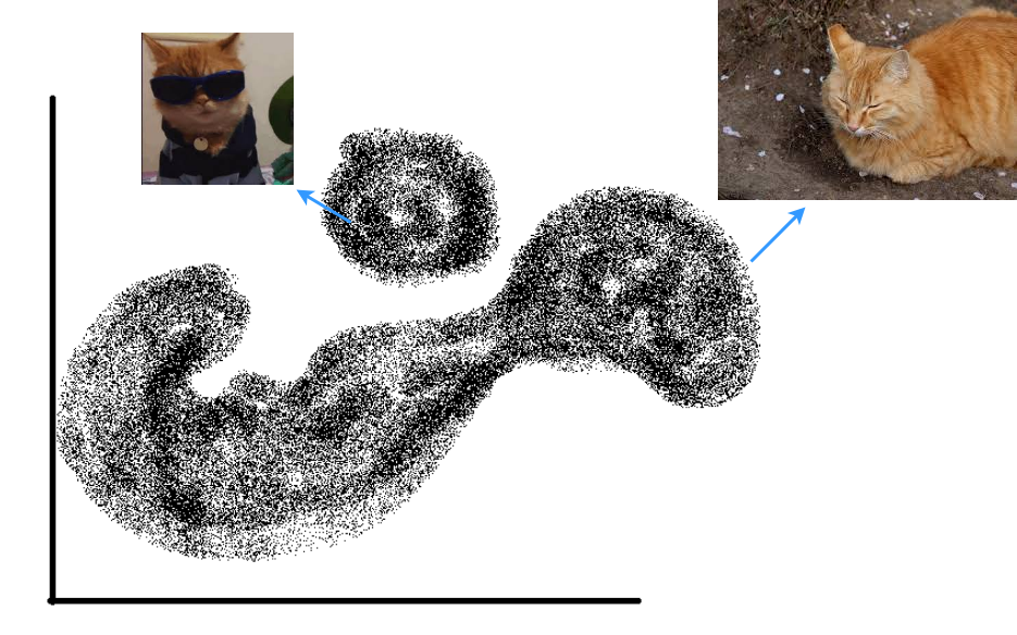
The -- 2D projection of the -- subspace of cat images where each point is a vector representing a cat picture. The probability density is implicit in the density of the actual data in the space (regions with more samples together are high probability and the white space is essentially zero probability).
There are two main families of generative models. Ones that directly learn the underlying probability density of the data (likelihood-based methods) and ones that learn the sampling process from the underlying probability density of the data (implicit generative models) [Song, and Ermon, (2019)]. This article focuses on the latter kind.
Boltzmann Distribution & Score-Based Models
The Boltzmann distribution is a probability distribution originating fron statistical physics that models the probability of a random variable in relation to its sampled value. Generative models leverage this distribution by associating the likelihood of data samples to scalar values called their “energy”. The following paragraph provides further intuition on this distribution.
Say I have a balloon filled with atoms of some atomic gas (Helium maybe) at temperature \(K\). I know that there are \(N\) atoms in the balloon. The temperature of a gas in a volume is the average kinetic energy of all atoms in that volume 2. Knowing that the average energy is \(K\), I want to know what is the energy of each atom in this balloon. This might be very very difficult to compute exactly. What if I pose this problem as what is the probability that a certain atom in this balloon has energy \(E(He)\). This is much easier to compute and the probability distribution of the energy of atoms in a gas is given by the Maxwell-Boltzmann Distribution.
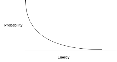
Boltzmann distribution for the energy of Helium atoms.
Formally, the Boltzmann distribution is a probability distribution that gives the probability that a system will be in a certain state, given the “energy” of that state. A general form of this for any (even non-physical) system is the Gibbs measure.
\[P(X = x) = \frac{e^{-E(x)}}{Z}\]Here, \(P\) is the probability that some vector \(x \in X\) has energy \(E(x)\). \(Z\) is a normalising factor that makes sure that the probability \(P\) of all such samples \(x\) adds up to 1 (\(\int P(x) dx = 1\)).
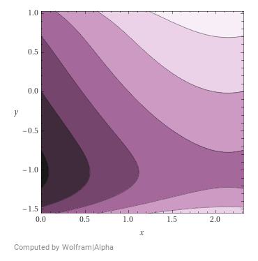
Energy function for some hypothetical 2D projection of a space of cat images.
Why is the energy function relevant? It can be argued that learning such an energy function for a dataset of samples is more tractable than learning the probability density function (this argument is solidified mathematically in the next subsection). We can assume that there exists some energy function that assigns low energy to vectors of cat images \(x\) in our subspace of cat images \(X\) and high energy to any other sample. Say, the energy function \(E(x)\) looks something like the following where dark regions indicate high energy (more likely that a sample does not exist here). It is necessary for the probability density function \(p(x)\) to add to 1 across all samples \(x \in X\). While no such requirement exists for an energy function. It is hence easier to learn this energy function using neural networks than it is to learn the probability density function.
Score-Based Models
The following excerpt is taken from [Song, and Ermon, (2019)] as I think it very clearly explains the mathematics of score-based models.
Suppose we are given a dataset \(\{ x_1, x_2, x_3, .. , x_N \}\) where each point is drawn independently from an underlying data distribution \(p(x)\). Given this dataset, the goal of generative modelling is to fit a model to the data distribution such that we can synthesize new data points at will by sampling from the distribution. To build such a generative model, we first need a way to represent a probability distribution. One such way, as in likelihood-based models, is to directly model the probability density function (p.d.f.) or probability mass function (p.m.f.).
Let \(f_{\theta}(x) \in R\) be a real-valued function (think of this as an energy function which is also called an unnormalised probabilistic model) parameterized by a learnable parameter \(\theta\). We can define the p.d.f of data points with energy \(f_{\theta}(x)\) using the Gibbs measure as
\(p_{\theta}(x) = \frac{e^{-f_{\theta}(x)}}{Z_{\theta}}\) where, \(Z_{\theta} > 0\) is the normalising constant. Likelihood-based methods find these parameters \(\theta\) by maximising the log-likelihood of the data \(\{ x_1, x_2, x_3, .. , x_N \}\).
\[\text{argmax}_{\theta} \sum_{i=1}^{N} \log p_{\theta(x_i)}\]However, maximising the log-likelihood requires the probability distribution \(p_{\theta}(x)\) to be normalised. Figuring out this normalising factor \(Z_{\theta}\) is typically intractable. This means that likelihood-based models are often restricted. This is where score-based models come in. We define the score as the gradient of the log probability \(p_{\theta}(x)\)
\(\begin{eqnarray} \text{score function} &=& \nabla_{x} \log(p(x)) \nonumber \\ &=& \nabla_{x} \log (\frac{e^{-f_{\theta}(x)}}{Z_{\theta}}) \nonumber \\ &=& \nabla_{x}(-f_{\theta}(x) - \log (Z_{\theta})) \nonumber \\ &=& -\nabla_{x} f_{\theta}(x) - 0 \nonumber \\ &=& -\nabla_{x}f_{\theta}(x) \nonumber \end{eqnarray}\) 3
To provide further intuition behind the score function, consider a single data sample from the cat distribution that has some amount of noise added to it. The noisy sample is shown below in green and its original position in the data distribution is shown in black. Further, the underlying energy function is shown as a contour in the background with light colours indicating low energy. As shown above, the gradient of the log probability of the sample with respect to the sample is the negative gradient of the energy of the sample with respect to the sample. This gradient is the direction of the steepest increase in the log probability which is also the direction of the steepest descent of the sample’s energy. In essence, the score is a denoising vector – which is the gradient of the log probability of the sample which is also the negative gradient of energy of the sample (w.r.t the sample) – that returns the noisy sample back to its position in the distribution.
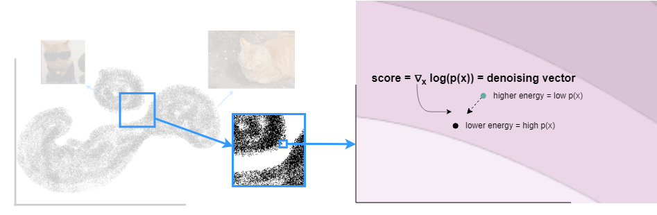
Score function in the cat space.
By modelling the score function instead of the density function, we can sidestep the difficulty of intractable normalizing constants. This means that a score-based model is independent of the normalising factor! This significantly expands the family of models that we can tractably use, since we don’t need any special architectures to make the normalizing constant tractable. Similar to likelihood-based models, we can train score-based models by minimizing the Fisher divergence between the model and the data distributions. If \(s_{\theta}(x)\) is the score-based model (which learns the score function to return the score for a sample \(x\) with energy \(f_{\theta}(x)\)), we learn the score function by minimising \(\mathbb{E}_{p_{x}} [\mathcal{L}2(\nabla_{x}p(x), s_{\theta}(x))]\). Of couse, we don’t know the true distribution \(p(x)\) (otherwise this whole thing is futile). We hence use score-matching to figure out the optimisation target. Score matching objectives can directly be estimated on a dataset and optimized with stochastic gradient descent, analogous to the log-likelihood objective for training likelihood-based models (with known normalizing constants). We can train the score-based model by minimizing a score matching objective, without requiring adversarial optimization.
Score Matching
The score is the gradient of the log probability of a sample (which is the negative gradient of the energy function). We aim to learn this score parameterised by parameters \(\theta\). To do this we can minimise the Fisher divergence between the gradient of the log probability w.r.t the data sample and the output of our model (which is the negative gradient of the energy).
\(s_{\theta}(x) =\) what we learn using gradient descent on the Fisher divergence (we learn a “good” \(\theta\)) \(= -\nabla_{x}f_{\theta}(x)\). The Fisher divergence is given by
\[\frac{1}{2} \mathbb{E}_{p_{\text{data}}} [\lVert\nabla_{x}\log(p_{\text{data}}(x)) - \nabla_{x}\log(p_{\theta}(x))\rVert^2]\]Intuitively, this means that given that you draw samples from a data distribution, you want to minimise the expectation (sum of some quantity over all samples) of the square of the L2 norm (distance) of the log probability of that sample having come from the data distribution and the log probability of that sample having come from your learnt distribution. You do this minimisation by tweaking your \(\theta\). In the end, you learn “good” parameters \(\theta\) such that the Fisher divergence is very close to zero.
But hold on, the Fisher divergence takes in the gradient of the log probability of the data distribution. We don’t know the data distribution!
Denoising Score Matching
Denoising score matching (DSM) [Vincent, (2011)] is an analogy between denoising autoencoders and the score function. In general, a denoising autoencoder aims to convert a noisy sample \(\tilde{x}\) back to its original form \(x\) by learning the added noise. Just like the example in the previous figure, say we have perturbed a sample from our distribution by adding some amount of Gaussian noise controlled by some variance.
\(\tilde{x} = x + \epsilon\) where \(\epsilon \sim \mathcal{N}(0, \sigma^2 \mathbb{I})\)
The score matching objective (Fisher divergence) can then be defined with respect to this noisy distribution as
\[\frac{1}{2} \mathbb{E}_{p_{\tilde{x}}} [\lVert \nabla_{\tilde{x}}\log(p_{\tilde{x}}(\tilde{x})) - s_{\theta}(\tilde{x})\rVert^2]\][Vincent, (2011)] show that this objective can be rewritten in terms of the conditional probability of sampling \(\tilde{x}\) given \(x\). The objective for DSM is hence
\[\frac{1}{2} \mathbb{E}_{p_{\tilde{x}, x}} [\lVert \nabla_{\tilde{x}}\log(p_{\tilde{x}, x}(\tilde{x} | x)) - s_{\theta}(\tilde{x})\rVert^2]\]The benefit of this is that while \(\nabla_{\tilde{x}} \log p_{\tilde {x}}(\tilde{x})\) is complex and can not be evaluated analytically , \(p_{\tilde{x}, x}(\tilde{x} \vert x)\) is a normal distribution which can be analytically evaluated. Intuitively, the gradient corresponds to the direction of moving from \(\tilde{x}\) back to the original \(x\) (i.e., denoising it), and we want our score-based model \(s_{\theta}(\tilde{x})\) to match that as best as it can.
References
Song, Yang and Ermon, Stefano (2019). Generative modeling by estimating gradients of the data distribution. Advances in neural information processing systems
Vincent, Pascal (2011). A connection between score matching and denoising autoencoders. Neural computation